191014K02 | Day 2 Lecture 1

191014K02: Day 2 Lecture 1

Back to the Course Page

Vertex Cover

Vertex Cover [Optimization]

Input: A graph $G = (V,E)$.

Task: Find $S \subseteq V(G)$ such that for all edges $(u,v) \in E(G)$, $\{u,v\} \cap S \neq \varnothing$ and minimize $|S|$.

Vertex Cover [Decision Version Edition]

Input: A graph $G = (V,E)$ and $k \in \mathbb{Z}^+$.

Task: Find $S \subseteq V(G)$ such that for all edges $(u,v) \in E(G)$, $\{u,v\} \cap S \neq \varnothing$ and $|S| \leqslant k$.

The naive algorithm by brute force — examining all possible subsets — is $O(n^k \cdot m)$ in damages. Can we do better?

The answer turns out to be yes: we can improve from $O(n^k \cdot m)$ to deterministic $2^k \cdot n^{O(1)}$ time, which is fixed-parameter tractable in $k$.

Having said that, we will begin with a very elegant randomized algorithm for Vertex Cover, which essentially picks an edge at random and then, one of its endpoints at random, for as long as it can.

Cute randomized algorithm ALG

$S=\varnothing$

while $G-S$ has at least one edge:

• pick $u,v \in E(G-S)$ u.a.r.
• pick $s \in\{u,v\}$ u.a.r
• Set $S \leftarrow S \cup\{s\}$

Output $S$

Here are few claims about cute algorithm:

1. ALG always runs in polynomial¹ time.
2. $S$ is always a vertex cover.
3. $\operatorname{Pr}$[$S$ is an optimal vertex cover] $\geqslant 1/2^k$.

The first two claims follow quite directly from the operations of the algorithm and the definition of a vertex cover.

What about the third? Well: let OPT be some fixed optimal vertex cover. Suppose $|$OPT$| \leqslant k$. Initially, note that $S \subseteq$ OPT. In each round, $\operatorname{Pr}$[$s \in S$] $\geqslant 1/2$, since $S \cap \{u,v\} \neq \varnothing$ by definition. If $s \in$ OPT in every round of the algorithm, then $S =$ OPT, which is awesome: and said awesomeness manifests with probability $1/2^k$.

Bonus: repeat the algorithm and retain the smallest solution to get an overall constant success probability:

$$1-\left(1-\frac{1}{2^k}\right)^{2^k} \geqslant 1-1 / e.$$

Approximation. Do we expect ALG to be a reasonable approximation? It turns out: yes!

In particular: we will show that the size of the vertex cover output by ALG is at most twice $|$OPT$|$ in expectation.

For a graph $G$, define $X_G$ to be the radom variable returning the size of the set $S$ output by the algorithm.

For integers $k,n$ define: $$X_{n,k}=\max_G E[X_G],$$

where the $\max$ is taken over all graphs with $\leqslant n$ vertices² and vertex cover of size $\leqslant k$.

Now let’s analyze the number $X_{n,k}$. Let $G^\star$ be the “worst-case graph” that bears witness to the $\max$ in the definition of $X_{n,k}$. Run the first step of ALG on $G^\star$. Suppose we choose to pick ${\color{indianred}s}$ in this step. $$\begin{aligned} X_{n,k}=E[X_{G^\star}] & = {\color{indianred}1}+\left(\frac{1}{2}+\varepsilon \right) E\left[{\color{darkseagreen}X_{G^\star-s} \mid s \in \text{OPT}}\right]+\left(\frac{1}{2} - \varepsilon\right) E\left[{\color{palevioletred}X_{G^\star-s} \mid s \notin \text {OPT}}\right] \\ & = 1 + \left(\frac{1}{2} + \varepsilon \right){\color{darkseagreen}X_{n, k-1}}+ \left(\frac{1}{2} - \varepsilon \right){\color{palevioletred}X_{n-1, k}}\\ & \leqslant 1 + \left(\frac{1}{2} + \varepsilon \right){\color{darkseagreen}X_{n, k-1}}+ \left(\frac{1}{2} - \varepsilon \right){\color{dodgerblue}X_{n, k}}\\ & = 1 + \frac{1}{2} X_{n, k-1} + \varepsilon \cdot X_{n, k-1} + \frac{1}{2} X_{n, k} - \varepsilon X_{n, k}\\ & \leqslant 1 + \frac{1}{2} X_{n, k-1} + \varepsilon \cdot {\color{dodgerblue}X_{n, k}} + \frac{1}{2} X_{n, k} - \varepsilon X_{n, k}\\ & = 1 + \frac{1}{2} X_{n, k-1} + {\color{indianred}\varepsilon \cdot X_{n, k}} + \frac{1}{2} X_{n, k} - {\color{indianred}\varepsilon X_{n, k}}\\ & = 1 + \frac{1}{2} X_{n, k-1} + \frac{1}{2} X_{n, k} \end{aligned}$$

Note that:

• $X_{n,k} \geqslant X_{n-1,k}$ and $X_{n,k} \geqslant X_{n,k-1}$.
• $\operatorname{Pr}[s \in \text{OPT}] \geqslant \frac{1}{2}$, in particular we let $\operatorname{Pr}[s \in \text{OPT}] = \frac{1}{2} + \varepsilon$.
• $\operatorname{Pr}[s \notin \text{OPT}] = 1 - \operatorname{Pr}[s \in \text{OPT}] = \frac{1}{2} - \varepsilon$.
• ${\color{darkseagreen}G^\star-s}$ is a graph on at most ${\color{darkseagreen}n}$ vertices with a vertex cover of size ${\color{darkseagreen}\leqslant k-1}$
• ${\color{palevioletred}G^\star-s}$ is a graph on at most ${\color{palevioletred}n}$ vertices with a vertex cover of size ${\color{palevioletred}\leqslant k}$

Rearranging terms, we get:

$$\frac{1}{2} X_{n,k} \leqslant 1 + \frac{1}{2} X_{n,k-1} \equiv X_{n,k} \leqslant 2 + X_{n,k-1}$$

Expanding the recurrence, we have: $X_{n,k} \leqslant 2k$, as claimed earlier.

Feedback Vertex Set

Now we turn to a problem similar to vertex cover, except that we are “killing cycles” instead of “killing edges”.

Feedback Vertex Set

Input: A (multi-)³graph $G = (V,E)$.

Task: Find $S \subseteq V(G)$ such that $G \setminus S$ is a forest⁴, and minimize $|S|$.

If we try to mimic the cute algorithm from before, we might easily be in trouble: note that the driving observation — that an edge has at least one of its endpoints in the solution with a reasonable enough probability — can fail spectacularly for FVS:

An example showing that for “most edges”, both endpoints do not belong to an optimal solution.

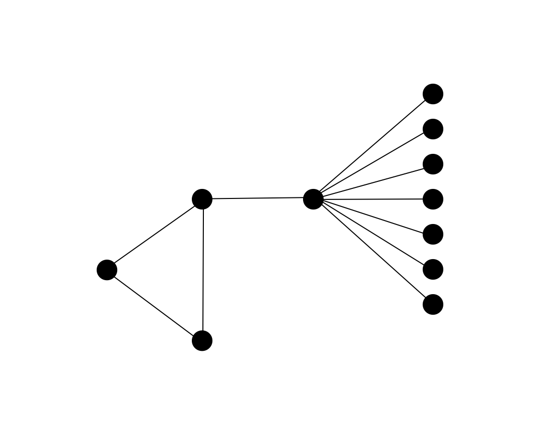
One thing about this example is the large number of pendant vertices sticking out prominently, and these clearly contribute to the badness of the situation. Happily, it turns out that we can get rid of these:

Lemma 1. Delete pendant and isolated vertices

Let $G$ be a multi-graph and $v$ be a vertex of degree $\leqslant 1$. Then:

• MinFVS of $G-\{v\}$ $\leqslant$ MinFVS of $G$

• $\forall S \subseteq V(G)-\{v\}$: $S$ is an FVS for $G$ $\leftrightarrow$ $S$ is an FVS for $G \setminus \{v\}$

Consider graphs with no pendant vertices and fix an optimal FVS $S$. Is it true that a reasonable fraction of edges are guaranteed to be incident to $S$? Well… not yet:

Spoiler

An(other) example showing that for “most edges”, both endpoints do not belong to an optimal solution, even though the graph has no pendant vertices.

However, continuing our approach of conquering-by-observing-patterns-in-counterexamples, note that the example above has an abundance of vertices that have degree two. Can we get rid of them? Well, isolated and pendant vertices were relatively easy because they don’t even belong to cycles, but that is not quite true for vertices of degree two. Can we still hope to shake them off?

One thing about a degree two vertex $u$ is that if there is a cycle that contains $u$ it must contain both its neighbors⁵. So you might suggest that we can ditch $u$ and just work with its neighbors instead. This intuition, it turns out, can indeed be formalized:

Lemma 2. Short-Circuiting Degree Two Vertices

Let:

• $G$ be a multi-graph,
• $u$ be a vertex of degree 2 that is not a self-loop,
• $a$ and $b$ be the neighbors of $u$ ($a=b$ is possible).

Let $H$ be the graph obtained by adding an edge $(a,b)$ to $G-\{u\}$.

Then:

• every FVS $S$ of $G$ such that $u \notin S$ is an FVS of $H$, and
• every FVS $S$ of $H$ is an FVS of $G$.

Illustrating Lemma 2 scenarios.

Let us also get rid of self-loops (because we can):

Lemma 3. Removing self-loops

If $G$ has a vertex $v$ with a self loop then

• Every FVS $S$ of $G$ contains $v$
• For every $S$ containing $v$: $S$ is an FVS of $G$ $\leftrightarrow$ $S-v$ is an FVS of $G-\{v\}$

Now let’s apply Lemmas 1—3 exhaustively, which is to say we keep applying them until none of them are applicable (as opposed to applying them until we feel exhausted ). Once we are truly stuck, we have a graph $H$ that is: (a) a graph whose minimum degree is three; and (b) equivalent to the original $G$ in the sense that any minimum FVS for $H$ can be extended to a minimum FVS of $G$ by some time travel: just play back the applications of Lemmas 1—3 in reverse order.

Recall that all this work was to serve our hope for having a cute algorithm for FVS as well. Let’s check in on how we are doing on that front: consider graphs whose minimum degree is three and fix an optimal FVS $S$. Is it true that a reasonable fraction of edges are guaranteed to be incident to $S$? Or can we come up with examples to demonstrate otherwise?

This is a good place to pause and ponder: play around with examples to see if you can come up with bad cases as before. If you find yourself struggling, it would be for a good reason: we actually now do have the property we were after! Here’s the main claim that we want to make.

Key Lemma

Let:

• $G$ be a multigraph with no self loops and minimum degree $\geqslant 3$,
• $S$ be an FVS of $G$,
• $(u,v)$ be a random edge in $E(G)$.

Then:

$\operatorname{Pr}[{\color{indianred}\{u, v\} \cap S \neq \varnothing}] \geqslant 1/2$

We argue this as follows: call an edge good if it has at least one of its endpoints in $S$, and bad otherwise.

We will demonstrate that the number of good edges is at least the number of bad edges: this implies the desired claim.

• The bad edges. Let $X := G \setminus S$. The bad edges are precisely $E(G[X])$.

• The good edges. Every edge that has one of its endpoints in $X$ and the other in $S$ is a good edge. Recall that $G$ has minimum degree three, because of which:

  • for every leaf in $G[X]$, we have at least two good edges, and
  • for vertex that is degree two in $G[X]$, we have at least one good edge.

So at this point, it is enough to show that twice the number of leaves and degree two vertices is at least $|E(G[X])| = |X|-1$. But this is quite intuitive if we simple stare at the following mildly stronger claim:

$$2 \cdot (\text{\# leaves}) + \text{\# deg-} 2 \text{vertices} \geqslant |X|$$

which is equivalent to:

$$2 \cdot ({\color{darkseagreen}\text{\# leaves}}) + {\color{palevioletred}\text{\# deg-}2 \text{vertices}} \geqslant ({\color{darkseagreen}\text{\# leaves}}) + {\color{palevioletred}\text{\# deg-}2 \text{ vertices}} + \text{\# deg-}(\geqslant 3) \text{ vertices}.$$

After cancelations, we have:

$$(\text{\# leaves}) \geqslant \text{\# deg-}(\geqslant 3) \text{ vertices}.$$

Note that this is true! Intuitively, the inequality is suggesting every branching vertex in a tree pays for at least one leaf — this can be formalized by induction on $n$.

Induction proof sketch

Denote the tree by $G$ and remove a leaf $u$ to obtain $H$. Apply the induction hypothesis on $H$.

• If the neighbor of $u$ in $G$ is a degree two vertex, then the number of leaves and high degree vertices are the same in $G$ and $H$, so the claim follows directly.
• If the degree of the neighbor in $u$ is three in $G$, then both quantities in the inequality for $H$ increase by one when we transition from $H$ to $G$.
• In the only remaining case, the quantity on the left increases by one when we come to $G$, which bodes well for the inequality.

All this was leading up to cute randomized algorithm v2.0 — i.e, adapted for FVS as follows:

Cute randomized algorithm redux

ALG$(G)$

Preprocess:

• if $G$ is acyclic return $\varnothing$
• if $\exists$ a self loop $v$ RETURN $($ALG$(G \setminus \{v\})) \cup \{v\}$.
• if $\exists$ a degree one vertex $v$ RETURN ALG$(G-\{v\})$.
• if $\exists$ a degree two vertex $v$ RETURN ALG$(G/\{v\})$ (c.f. Lemma 2).

---

Mindeg-3 instance:

• pick an edge $(u,v) \in E(G)$ u.a.r.
• pick $s \in \{u,v\}$ u.a.r.
• RETURN $($ALG$(G \setminus \{s\})) \cup \{s\}$

Claim 1

ALG always returns a FVS of $G$.

This follows from Lemmas 1—3 and induction on $n$.

Claim 2

If $G$ has a FVS of size $k$, then $\operatorname{Pr}$[ALG returns an optimal FVS] $\geqslant 1/4^k$.

This follows from Lemmas 1—3, the key lemma, and induction on $n$.

Exact Algorithms

Coming Soon.

Footnotes

1. (even linear)

2. We could have also considered $X_k = \max_G E[X_G]$, where the max is over all graphs whose vertex cover is at most $k$: but there are infinitely many graphs that have vertex covers of size at most $k$, and it is not immediate that the max is well-defined, so we restrict ourselves to graphs on $n$ vertices that have vertex covers of size at most $k$.

3. We allow for more than one edge between a fixed pair of vertices and self-loops.

4. A graph without cycles that is not necessarily connected.

5. Except when the cycle only contains $u$, i.e, $u$ has a self-loop.